Estimating qpmR models: priors, posteriors, identification • qpmR

qpmR estimates any subset of structural parameters and shock standard deviations by Bayesian methods (or maximum likelihood) over the Kalman-filter likelihood of the solved model. Everything without a prior stays calibrated – the operational reality of semi-structural models, where a handful of transmission parameters are estimated and the rest are judgmental.

Priors

priors() provides a small language in the mean/sd parametrization economists write down. The distribution constructors exist only inside priors(), so base R’s beta() and gamma() functions are never masked:

library(qpmR)
#> 
#> Attaching package: 'qpmR'
#> The following object is masked from 'package:stats':
#> 
#>     var
pr <- priors(
  rho = beta(0.5, 0.2),
  e   = invgamma(1, 0.5)    # a shock name means that shock's sd
)
pr
#> <qpm_priors> 2 priors
#>   rho        beta(mean  0.5, sd  0.2) on (0,    1)
#>   e          invgamma(mean    1, sd  0.5) on (0,  Inf)

truncate(normal(1.5, 0.25), lower = 1) restricts support (and renormalizes, so marginal likelihoods remain valid).

A laboratory: estimating an AR(1)

Simulate data from a known truth, then ask the posterior to find it:

m0 <- qpm_model(variables = vars(x = "x"), shocks = shocks(e),
                equations = eqs(x ~ rho * x[-1] + e),
                params = list(rho = 0.5))
m_true <- qpm_calibrate(m0, rho = 0.8, sigma = c(e = 1.5))
obs <- simulate(qpm_solve(m_true), nsim = 250, seed = 4)

est <- qpm_estimate(m0, obs, pr, iter = 800, chains = 2, seed = 5,
                    verbose = FALSE)
est
#> <qpm_estimate> Bayesian (adaptive RWM) - 2 parameters, 2 chains x 800 draws (burn 400, acceptance 0.28)
#>   log-posterior at mode: -444.29
#>   param      prior                  mode     mean       5%      95%  R-hat    ESS learned
#>   rho        beta(0.5, 0.2)        0.750    0.745    0.688    0.800   1.02    102 yes
#>   e          invgamma(1, 0.5)      1.413    1.418    1.334    1.518   1.02    108 yes
#>   'learned' compares posterior to prior sd (yes < 0.5 < some < 0.9 < little)

The sampler finds the posterior mode first (in transformed, unconstrained space), seeds an adaptive random-walk Metropolis with the inverse Hessian, and reports split R-hat and effective sample sizes. The learned column compares posterior to prior spread – a cheap identification signal. Draws that violate Blanchard-Kahn get zero weight, which is the usual truncation of the prior to the determinacy region.

plot(est)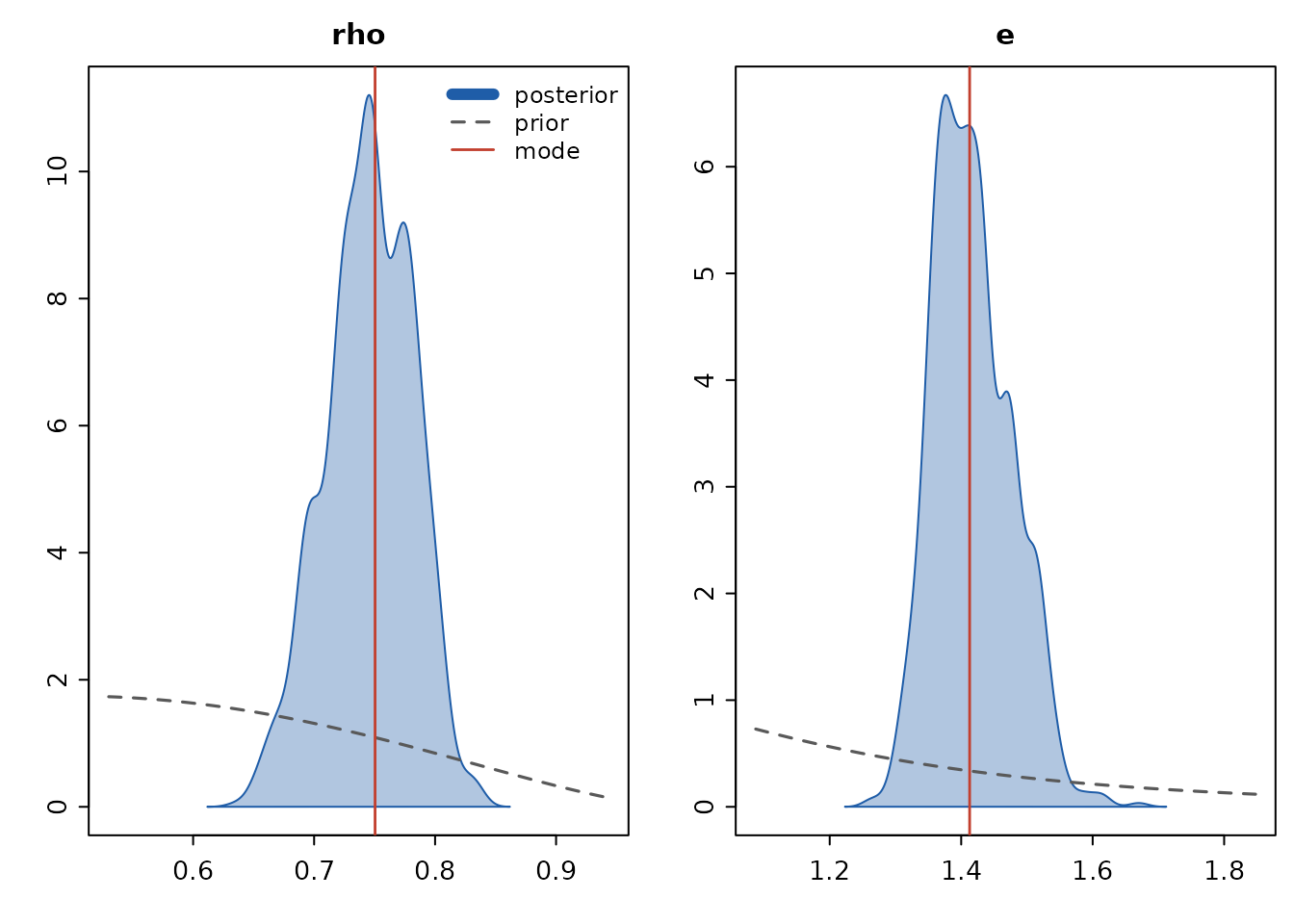

Point estimates feed straight back into the workflow:

m_hat <- apply_estimate(est, "mean")
round(coef(est, "mean"), 3)
#>   rho     e 
#> 0.745 1.418

And posterior_forecast() produces fans that integrate over the posterior – each draw re-solves the model and re-filters the data, so the bands combine shock and parameter uncertainty:

fc <- posterior_forecast(est, horizon = 10, ndraws = 80)
plot(fc, vars = "x")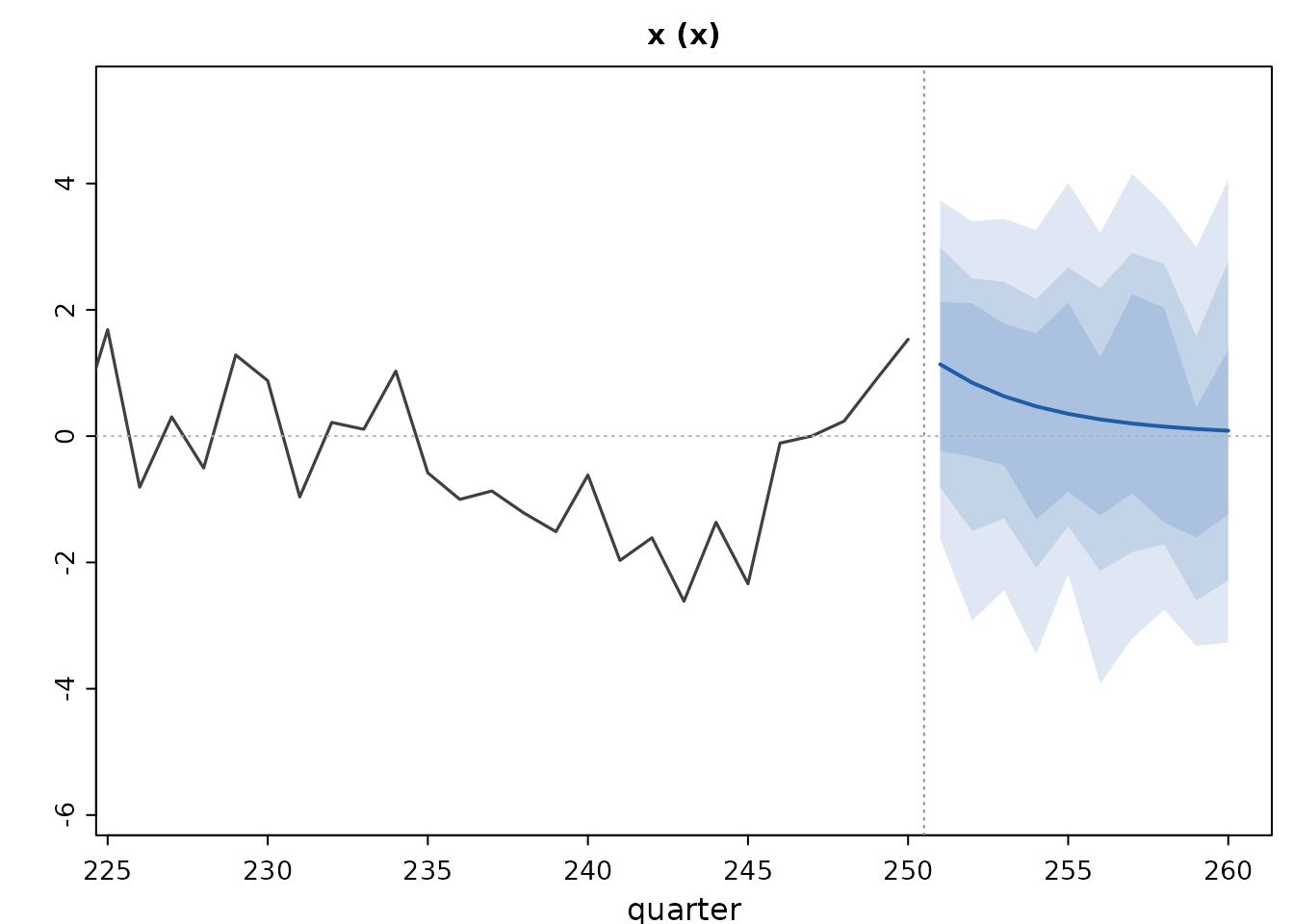

Identification: ask before you sample

qpm_identify() checks, before any MCMC, whether the chosen parameters can be told apart – numerically differentiating the solved model and its population moments in the spirit of Iskrev (2010). A model in which two parameters enter only as a product is the classic failure:

m_bad <- qpm_model(variables = vars(x = "x"), shocks = shocks(e),
                   equations = eqs(x ~ a * b * x[-1] + e),
                   params = list(a = 0.6, b = 0.9))
qpm_identify(m_bad, params = c("a", "b"))
#> <qpm_identification> 2 parameters, observables: x
#>   x solution level: rank 1 < 2 - parameters not separately identified
#>       combinations involved: a, b
#>   ! solution level: near-collinear pairs (only jointly identified): a ~ b (1.000)
#>   x moment level (means + autocovariances to lag 3): rank 1 < 2 - parameters not separately identified
#>       combinations involved: b, a
#>   ! moment level (means + autocovariances to lag 3): near-collinear pairs (only jointly identified): a ~ b (1.000)

On the template, the core transmission parameters pass at full rank:

qpm_identify(qpm_template("bkl"),
             params = c("b1", "b2", "b3", "c1", "c2", "a1", "a3"),
             observables = c("pi", "i", "q", "y_gap", "dy_obs"))
#> <qpm_identification> 7 parameters, observables: pi, i, q, y_gap, dy_obs
#>   v solution level: full rank (7), smallest/largest singular value 0.045
#>   v moment level (means + autocovariances to lag 3): full rank (7), smallest/largest singular value 0.023

Marginal likelihood and Bayes factors

marginal_likelihood() reports the modified harmonic mean (Geweke 1999) across truncation probabilities, with a Laplace approximation as a cross-check. Differences across models on the same data are log Bayes factors:

ml_ar1 <- marginal_likelihood(est)
ml_ar1
#> <qpm_logml> log marginal likelihood: -448.42
#>   modified harmonic mean over 800 draws, 2 parameters
#>   by truncation: -447.85, -448.56, -448.63, -448.55, -448.51 (spread 0.77)
#>   Laplace approximation: -448.46
#>   differences across models on the same data are log Bayes factors

# a deliberately misspecified rival: white noise (rho fixed at 0)
est_wn <- qpm_estimate(qpm_calibrate(m0, rho = 0), obs,
                       priors(e = invgamma(1, 0.5)),
                       iter = 800, chains = 2, seed = 6, verbose = FALSE)
ml_wn <- marginal_likelihood(est_wn)
cat(sprintf("log Bayes factor, AR(1) vs white noise: %.1f\n",
            ml_ar1$logml - ml_wn$logml))
#> log Bayes factor, AR(1) vs white noise: 106.4

On real data

The same call estimates the Czech model shipped with the package. It takes minutes rather than seconds (each draw solves the model and filters 27 years of data), so it is not run here:

mcz <- qpm_calibrate(qpm_template("bkl", trends = "rw"),
                     pi_tar = 2, istar_ss = 2, pistar_ss = 2,
                     prem_ss = 1, a5 = 0.4)
cz <- czechia[czechia$period >= "1999",
              c("period", "pi4", "i", "q", "dy_obs", "istar", "pistar")]
est_cz <- qpm_estimate(mcz, cz, priors(
  b1 = beta(0.70, 0.10), b2 = gamma(0.25, 0.10), b3 = gamma(0.10, 0.05),
  c1 = beta(0.70, 0.10), c2 = truncate(normal(1.5, 0.25), lower = 1),
  eps_pi = invgamma(1.0, 0.5)
), iter = 3000, chains = 2, seed = 42)

Results from that run (2 chains x 3000 draws, acceptance 0.30):

param    prior                  mode   mean     5%    95%  R-hat  ESS  learned
b1       beta(0.7, 0.1)        0.378  0.380  0.342  0.417   1.01  226  yes
b2       gamma(0.25, 0.1)      0.050  0.058  0.033  0.089   1.01  101  yes
b3       gamma(0.1, 0.05)      0.003  0.005  0.002  0.010   1.01  100  yes
c1       beta(0.7, 0.1)        0.865  0.861  0.839  0.881   1.02  108  yes
c2       trunc-normal(1.5,.25) 1.352  1.282  1.017  1.726   1.26   17  little
eps_pi   invgamma(1, 0.5)      2.629  2.706  2.414  3.033   1.00   99  yes

The data speak loudly and say familiar things: inflation is far less intrinsically persistent than the canonical calibration (b1 0.38 vs 0.70), the Phillips curve is flat (b2 0.06), policy smoothing is high (c1 0.86), and the cost-push shock standard deviation nearly triples – the 2022-23 inflation crisis, quantified. The exception is honest too: c2, the rule’s inflation response, mixes poorly (R-hat 1.26, ESS 17) and piles against its Taylor-principle bound – response coefficients are weakly identified under high smoothing, and the diagnostics say so rather than reporting a confident point estimate.