Forecast error variance decomposition

Splits the forecast error variance of each variable at each horizon into the contributions of the structural shocks — "how much of inflation uncertainty two years out is the cost-push shock?". For $$x_t = P x_{t-1} + Q e_t, e_t ~ N(0, S)$$ the h-step forecast error variance is $$V_h = sum_{j<h} P^j Q S Q' (P^j)'$$ and the share of shock k is the same sum with only column k of Q active. Shares sum to one across shocks for every variable and horizon.

Usage

fevd(x, ...)

# S3 method for class 'qpm_solution'
fevd(x, horizon = 24, vars = NULL, shocks = NULL, ...)

# S3 method for class 'qpm_fevd'
plot(x, var = NULL, drop_zero = TRUE, ...)

Arguments

x: A qpm_solution, or a qpm_model (solved first).
...: Passed to methods.
horizon: Largest forecast horizon.
vars: Variables to include; default all declared variables.
shocks: Shocks to include; default all.
var: Variable to plot.
drop_zero: Omit shocks that never contribute.

Value

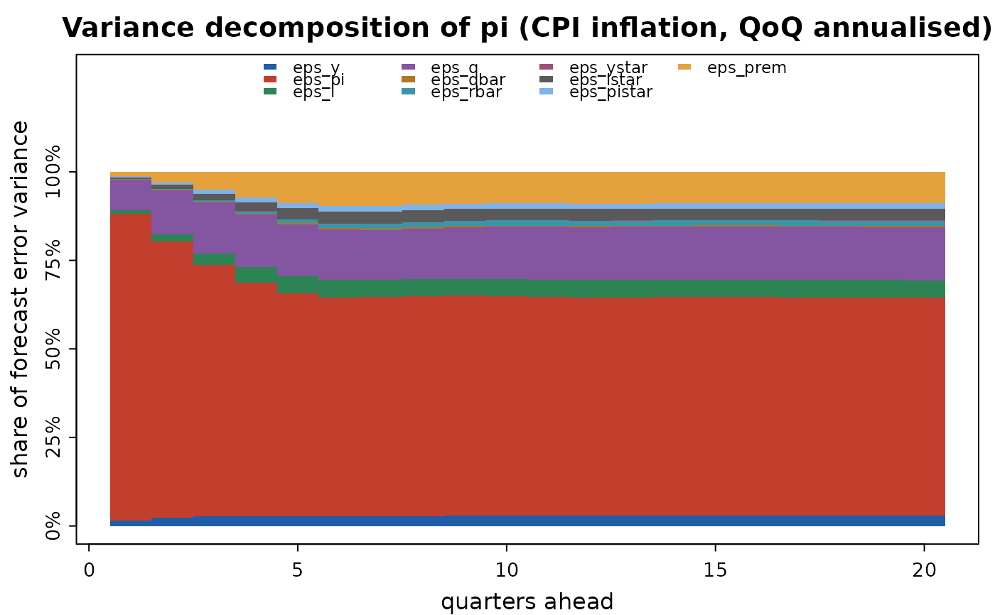
A data frame of class qpm_fevd in long format with columns variable, shock, horizon, share and variance. print() shows the dominant shocks; plot() draws stacked shares.

Details

Shares remain well defined when the model has unit roots, even though the variances themselves grow without bound.

Examples

sol <- qpm_solve(qpm_template("bkl"))
fv <- fevd(sol, horizon = 20)
fv
#> <qpm_fevd> Canonical small open economy QPM (BKL, stationary trends) - shares of forecast error variance
#>   horizons 1, 4, 8, 20; dominant shocks per variable:
#>     y_gap      eps_y 66%   eps_y 45%   eps_pi 41%   eps_pi 40%
#>     pi         eps_pi 87%   eps_pi 66%   eps_pi 62%   eps_pi 61%
#>     pi4        eps_pi 87%   eps_pi 70%   eps_pi 57%   eps_pi 57%
#>     i          eps_pi 40%   eps_pi 41%   eps_pi 33%   eps_pi 36%
#>     r          eps_pi 54%   eps_pi 51%   eps_pi 46%   eps_pi 47%
#>     r_gap      eps_pi 54%   eps_pi 52%   eps_pi 46%   eps_pi 46%
#>     q          eps_q 86%   eps_q 54%   eps_q 49%   eps_q 44%
#>     q_gap      eps_q 86%   eps_q 55%   eps_q 50%   eps_q 46%
#>     q_bar      eps_qbar 100%   eps_qbar 100%   eps_qbar 100%   eps_qbar 100%
#>     r_bar      eps_rbar 100%   eps_rbar 100%   eps_rbar 100%   eps_rbar 100%
#>     dy_obs     eps_y 57%   eps_y 50%   eps_y 44%   eps_y 38%
#>     dy_bar     eps_g 100%   eps_g 100%   eps_g 100%   eps_g 100%
#>     ystar_gap  eps_ystar 100%   eps_ystar 100%   eps_ystar 100%   eps_ystar 100%
#>     istar      eps_istar 100%   eps_istar 100%   eps_istar 100%   eps_istar 100%
#>     pistar     eps_pistar 100%   eps_pistar 100%   eps_pistar 100%   eps_pistar 100%
#>     rstar      eps_pistar 58%   eps_istar 51%   eps_istar 56%   eps_istar 57%
#>     prem       eps_prem 100%   eps_prem 100%   eps_prem 100%   eps_prem 100%
plot(fv, var = "pi")