qpm_diff() compares model structure — what a country team changed
in the code. This compares model behaviour: the transmission of a
given shock and the moments each specification implies. When a
calibration is revised, both questions matter, and the second is the
one a policy audience asks.
Usage
qpm_compare_models(models, shock = NULL, vars = NULL, horizon = 20)

# S3 method for class 'qpm_model_comparison'
plot(x, vars = NULL, ...)
Arguments
- models
A named list of
qpm_modelorqpm_solutionobjects.- shock
Shock whose impulse responses are compared. Default: the first shock common to every model.
- vars
Variables to compare. Default: those common to all models, capped at the usual headline set.
- horizon
Impulse-response horizon.
- x
A
qpm_model_comparison.- ...
Unused.
Value
An object of class qpm_model_comparison holding the
impulse responses and, for stationary models, the implied moments.
Examples
base <- qpm_template("bkl")
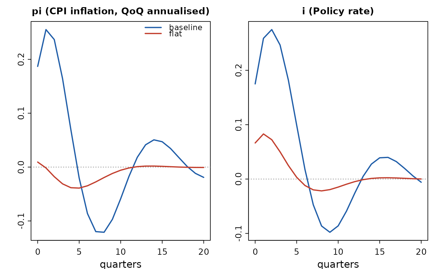
flat <- qpm_calibrate(base, b2 = 0.05)   # a much flatter Phillips curve
cmp <- qpm_compare_models(list(baseline = base, flat = flat),
                          shock = "eps_y")
cmp
#> <qpm_model_comparison> baseline vs flat
#>   response to eps_y over 20 quarters
#>   peak response by model:
#>     pi4        baseline +0.21@3   flat -0.04@6
#>     pi         baseline +0.26@1   flat -0.04@5
#>     i          baseline +0.27@2   flat +0.08@1
#>     y_gap      baseline +0.53@0   flat +0.50@0
#>     q          baseline -0.39@2   flat -0.20@1
#>   implied standard deviations:
#>     pi4        baseline 2.43   flat 1.86
#>     pi         baseline 2.89   flat 2.20
#>     i          baseline 2.50   flat 2.19
#>     y_gap      baseline 1.61   flat 1.72
#>     q          baseline 3.24   flat 3.21
plot(cmp, vars = c("pi", "i"))