Evaluate alternative policy rules

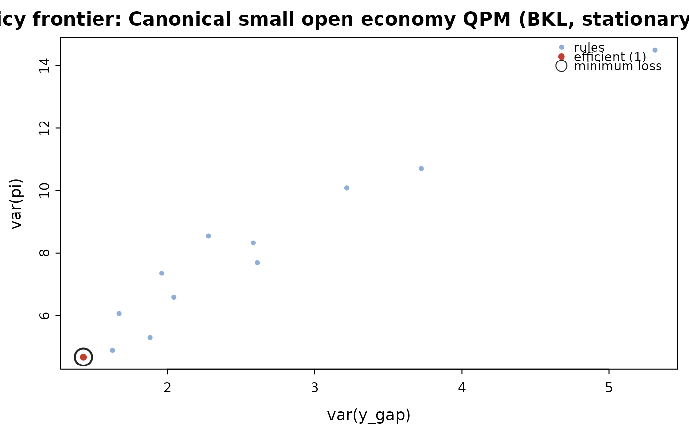
Answers the question a policy committee actually asks — what if we responded differently? — by re-solving the model over a grid of rule parameters and scoring each one by the unconditional loss $$L = sum_v w_v var(v) + sum_v w^d_v var(v - v_{-1})$$ computed from the model's stationary covariance rather than by simulation, so it is exact. Tracing the resulting variance pairs gives the inflation-output variability frontier (the Taylor curve).

Usage

qpm_rule_eval(model, grid, loss = c(pi = 1, y_gap = 0.5), diff_loss = NULL)

# S3 method for class 'qpm_rule_eval'
plot(x, xvar = NULL, yvar = NULL, ...)

Arguments

model

A qpm_model.

grid

A data frame of parameter values, one row per rule and one column per parameter (e.g. from expand.grid()).

loss

Named weights on the variances of levels, e.g. c(pi = 1, y_gap = 0.5).

diff_loss

Named weights on the variances of first differences, e.g. c(i = 0.5) to penalise instrument volatility.

x

A qpm_rule_eval.

xvar, yvar

Axes of the frontier. Either a variable name, whose level variance is used, or a scored column name directly — so xvar = "vard_i" traces the classic trade-off against instrument volatility. Defaults to the first two entries in loss.

...

Unused.

Value

A data frame of class qpm_rule_eval: the grid, the variance of each targeted variable, the loss, and the Blanchard-Kahn outcome.

Details

Rules that violate Blanchard-Kahn are reported as such rather than dropped: a policy response too weak to deliver determinacy is a finding, not a missing row.

Examples

m <- qpm_template("bkl")
grid <- expand.grid(c2 = c(1.2, 1.5, 2, 3), c3 = c(0, 0.5, 1))
ev <- qpm_rule_eval(m, grid, loss = c(pi = 1, y_gap = 0.5),
                    diff_loss = c(i = 0.5))
ev
#> <qpm_rule_eval> Canonical small open economy QPM (BKL, stationary trends) - 12 rules
#>   loss: 1*var(pi) + 0.5*var(y_gap) + 0.5*var(di)
#>   best 8 by loss:
#>  c2  c3  var_pi var_y_gap var_i vard_i loss  
#>  3.0 1.0 4.679  1.429     5.469 1.358   6.073
#>  3.0 0.5 4.896  1.627     5.298 1.305   6.362
#>  3.0 0.0 5.297  1.881     5.188 1.265   6.870
#>  2.0 1.0 6.067  1.670     5.948 1.285   7.545
#>  2.0 0.5 6.595  2.043     5.761 1.247   8.241
#>  1.5 1.0 7.358  1.963     6.460 1.287   8.982
#>  2.0 0.0 7.700  2.612     5.734 1.237   9.624
#>  1.5 0.5 8.332  2.585     6.272 1.268  10.258
plot(ev)