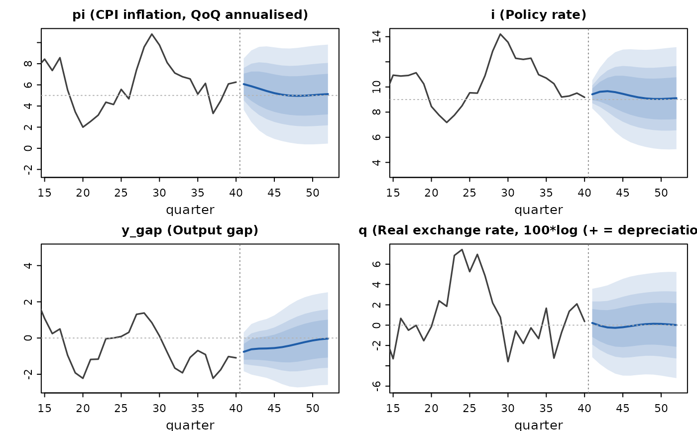
Model forecast with uncertainty bands — qpm

Iterates the solved model forward from an initial state and computes analytic forecast uncertainty from the shock variances, $$V_h = P V_{h-1} P' + Q S Q'$$ giving Gaussian fan bands around the mean path. The result can then be conditioned on assumed paths with qpm_condition(), shifted by shock scenarios with qpm_scenario(), or adjusted with logged judgment via add_judgment().

Usage

qpm_forecast(
  object,
  from = NULL,
  horizon = 12,
  bands = c(0.5, 0.7, 0.9),
  sigma = NULL
)

Arguments

object: A qpm_solution.
from: Initial state: a qpm_filtration from qpm_filter() (the smoothed end-of-sample state is used and the smoothed history is kept for plotting), a qpm_sim from simulate(), a full named deviation vector over object$vars_all, or NULL (steady state).
horizon: Forecast horizon in quarters.
bands: Coverage levels for the fan, e.g. c(0.5, 0.7, 0.9).
sigma: Optional named vector of shock standard deviations.

Value

An object of class qpm_forecast: a list with paths (long data frame: variable, h, mean, and lo_*/hi_* per band, in levels), forecast-period labels in $periods, plus the machinery needed for conditioning.

Examples

sol <- qpm_solve(qpm_template("bkl"))
histq <- simulate(sol, nsim = 40, seed = 7, burn = 20)
fc <- qpm_forecast(sol, from = histq, horizon = 12)
fc
#> <qpm_forecast> Canonical small open economy QPM (BKL, stationary trends) - 12 quarters ahead (h1 ... h12)
#>   mean (90% band) at h = 1, 4, 8, 12:
#>     y_gap      -0.76 (-1.83, 0.31)  -0.58 (-2.2, 1.05)  -0.32 (-2.73, 2.08)  -0.03 (-2.59, 2.53)
#>     pi         6.07 (3.64,  8.5)  5.42 (1.19, 9.64)  4.96 (0.42,  9.5)  5.13 (0.45, 9.81)
#>     pi4        5.73 (5.12, 6.34)  5.75 ( 2.8,  8.7)  5.06 (1.37, 8.75)  5.05 (1.13, 8.97)
#>     i          9.41 ( 8.3, 10.5)  9.59 (6.41, 12.8)  9.09 (5.23, 12.9)  9.11 (5.05, 13.2)
#>     r          3.55 (1.83, 5.26)  4.37 (2.12, 6.62)  4.11 (0.88, 7.33)  3.95 (0.56, 7.35)
#>     r_gap      -0.26 (-1.98, 1.46)  0.51 (-1.73, 2.75)   0.2 (-3.04, 3.44)  0.01 (-3.41, 3.44)
#>     q          0.22 (-3.15, 3.58)  -0.26 (-4.77, 4.24)   0.1 (-4.84, 5.04)  0.01 (-5.21, 5.23)
#>     q_gap      1.19 (-2.18, 4.56)  0.44 (-4.03, 4.92)  0.57 (-4.31, 5.44)  0.31 (-4.84, 5.47)
#>     q_bar      -0.97 (-1.47, -0.48)  -0.71 (-1.56, 0.15)  -0.47 (-1.49, 0.56)  -0.31 (-1.39, 0.78)
#>     r_bar      3.81 (3.48, 4.14)  3.86 (3.29, 4.43)  3.91 (3.23, 4.59)  3.94 (3.22, 4.66)
#>     dy_obs     4.63 (0.03, 9.24)  3.41 (-2.12, 8.94)  3.83 (-2.2, 9.86)  3.62 (-2.78,   10)
#>     dy_bar      3.3 (2.97, 3.63)  3.38 (2.85, 3.91)  3.44 (2.84, 4.04)  3.47 (2.85, 4.08)
#>     ystar_gap  -0.42 (-0.91, 0.07)  -0.21 (-0.96, 0.54)  -0.09 (-0.9, 0.72)  -0.04 (-0.86, 0.78)
#>     istar      3.53 (3.04, 4.03)  3.33 (2.53, 4.13)  3.17 (2.27, 4.07)  3.09 (2.16, 4.02)
#>     pistar     2.44 (1.62, 3.27)  2.15 (1.03, 3.27)  2.04 (0.89, 3.19)  2.01 (0.86, 3.16)
#>     rstar      1.22 (0.47, 1.98)  1.22 ( 0.1, 2.34)  1.15 (-0.06, 2.35)  1.08 (-0.15, 2.31)
#>     prem       2.89 (2.06, 3.71)  2.93 ( 1.6, 4.26)  2.96 (1.46, 4.47)  2.98 (1.44, 4.53)
plot(fc, vars = c("pi", "i", "y_gap", "q"))