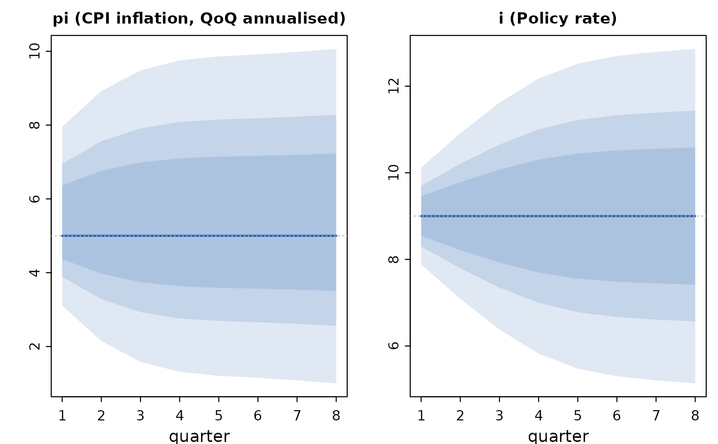
Central banks rarely believe their fan charts are symmetric: the
published judgement is usually "risks to inflation are tilted to the
upside". qpm_risk() applies that judgement, replacing the Gaussian
bands of a forecast with two-piece normal bands whose mode stays on
the model's projection while the mean shifts by the stated skew.
Total uncertainty is preserved: the variance implied by the model at
each horizon is held fixed, so a skew redistributes risk rather than
adding it.
Value
The forecast with skewed bands. $risk records the skews and
$paths gains a mode column alongside mean.
Details
The skew is stated in the variable's own units as mean minus mode —
a value of 0.3 on inflation means the risks are worth 0.3
percentage points to the upside. Skews may be given for any subset of
variables and horizons; anything unstated keeps symmetric bands.
Unlike add_judgment(), which moves the projection itself and
back-solves the shocks that support it, this changes only the shape of
the distribution around an unchanged central path.
Examples
sol <- qpm_solve(qpm_template("bkl"))
fc <- qpm_forecast(sol, horizon = 8)
risky <- qpm_risk(fc, pi = 0.4, author = "MPC",
                  rationale = "energy prices tilted to the upside")
risky
#> <qpm_forecast> Canonical small open economy QPM (BKL, stationary trends) - 8 quarters ahead (h1 ... h8)
#>   mean (90% band) at h = 1, 4, 8:
#>     y_gap      0 (-1.07, 1.07)  0 (-1.63, 1.63)  0 (-2.4,  2.4)
#>     pi          5.4 (3.11, 7.96)   5.4 (1.31, 9.75)   5.4 (   1, 10.1)
#>     pi4           5 (4.39, 5.61)     5 (2.05, 7.95)     5 (1.31, 8.69)
#>     i             9 (7.88, 10.1)     9 (5.82, 12.2)     9 (5.14, 12.9)
#>     r             4 (2.28, 5.72)     4 (1.75, 6.25)     4 (0.78, 7.22)
#>     r_gap      0 (-1.72, 1.72)  0 (-2.24, 2.24)  0 (-3.24, 3.24)
#>     q          0 (-3.37, 3.37)  0 (-4.51, 4.51)  0 (-4.94, 4.94)
#>     q_gap      0 (-3.37, 3.37)  0 (-4.47, 4.47)  0 (-4.87, 4.87)
#>     q_bar      0 (-0.49, 0.49)  0 (-0.85, 0.85)  0 (-1.02, 1.02)
#>     r_bar         4 (3.67, 4.33)     4 (3.43, 4.57)     4 (3.32, 4.68)
#>     dy_obs      3.5 (-1.11, 8.11)   3.5 (-2.03, 9.03)   3.5 (-2.53, 9.53)
#>     dy_bar      3.5 (3.17, 3.83)   3.5 (2.97, 4.03)   3.5 ( 2.9,  4.1)
#>     ystar_gap  0 (-0.49, 0.49)  0 (-0.75, 0.75)  0 (-0.81, 0.81)
#>     istar         3 (2.51, 3.49)     3 ( 2.2,  3.8)     3 ( 2.1,  3.9)
#>     pistar        2 (1.18, 2.82)     2 (0.88, 3.12)     2 (0.85, 3.15)
#>     rstar         1 (0.24, 1.76)     1 (-0.12, 2.12)     1 (-0.21, 2.21)
#>     prem          3 (2.18, 3.82)     3 (1.67, 4.33)     3 ( 1.5,  4.5)
#>   balance of risks: 8 entries on pi (see risk_log())
#>     bands are two-piece normal; the central line is the mode
plot(risky, vars = c("pi", "i"))